The science under Understory
Identification with a guarantee
Pulling a native plant by mistake is the costliest error a volunteer can make, and American bittersweet, staghorn sumac and black walnut all have invasive look-alikes. So Understory’s classifier gives one of four decisions. PULL means a core invasive target, DON’T PULL means a native or look-alike is most likely, and OTHER INVASIVE means a secondary invasive such as barberry or buckthorn. Otherwise it says INSPECT and asks for the view that settles it, such as where the fruit grows on a bittersweet vine.
A BioCLIP 2 foundation model, adapted with LoRA, is the teacher. It is distilled into BioCLIP’s much smaller ViT-B/16, which runs offline on an iPhone as a 57.9 MB Core ML model.
Everything is tested on a geographic holdout of every Massachusetts photo, 16,987 photos by 3,940 people, none of whom appears in training. The shipped threshold is calibrated on Massachusetts photos too, so its error rates come from cross-validation over map blocks. It is calibrated on four folds and tested on the fifth, with that fold’s photographers removed.
Invasive targets
4,733 photos
Look-alikes
4,494 photos
Other invasives
3,221 photos
Native plants
4,539 photos
The hardest case is highbush blueberry with red leaves in October, which looks like burning bush. Patch extent is measured without LiDAR: ARKit visual-inertial odometry plus Depth Anything V2 monocular depth, scale-aligned to ARKit’s feature points.
My field testing
My first review of field photos, taken at dusk, simply accepted the app’s suggestions, so I labeled every plant again without seeing its answers. On 126 plants at Turning Mill Pond and Wright Farm, the app caught 21 of 22 invasive targets and told just 1 of 82 natives and look-alikes to PULL, a raspberry shot at 4.7× zoom, so its camera now stops at 2×. It named the species right for 56 of the 61 plants it has a class for.
Seeing next year’s problem
Spread on a 2-meter grid
Each surveyed patch spreads in a stage-structured stochastic integrodifference model: plants grow in place, then seeds, fruit and rhizome fragments travel by each species’ dispersal kernel, with rare long jumps, and settle where the habitat allows. A Monte Carlo ensemble turns that into a probability of invasion for every 2 m cell, year by year, and into the area that clearing each patch would prevent. Every one of the model’s numbers cites its source in the literature.
The simulator is C++. The API runs it natively; the map runs the same code compiled to WebAssembly, so the impact of skipping a patch is simulated in your browser.
Understory’s integrodifference model fits in one line. Next year’s density of plants at a point adds up what this year’s plants produce at every point , carried to by the dispersal kernel , and keeps what the habitat lets settle there.
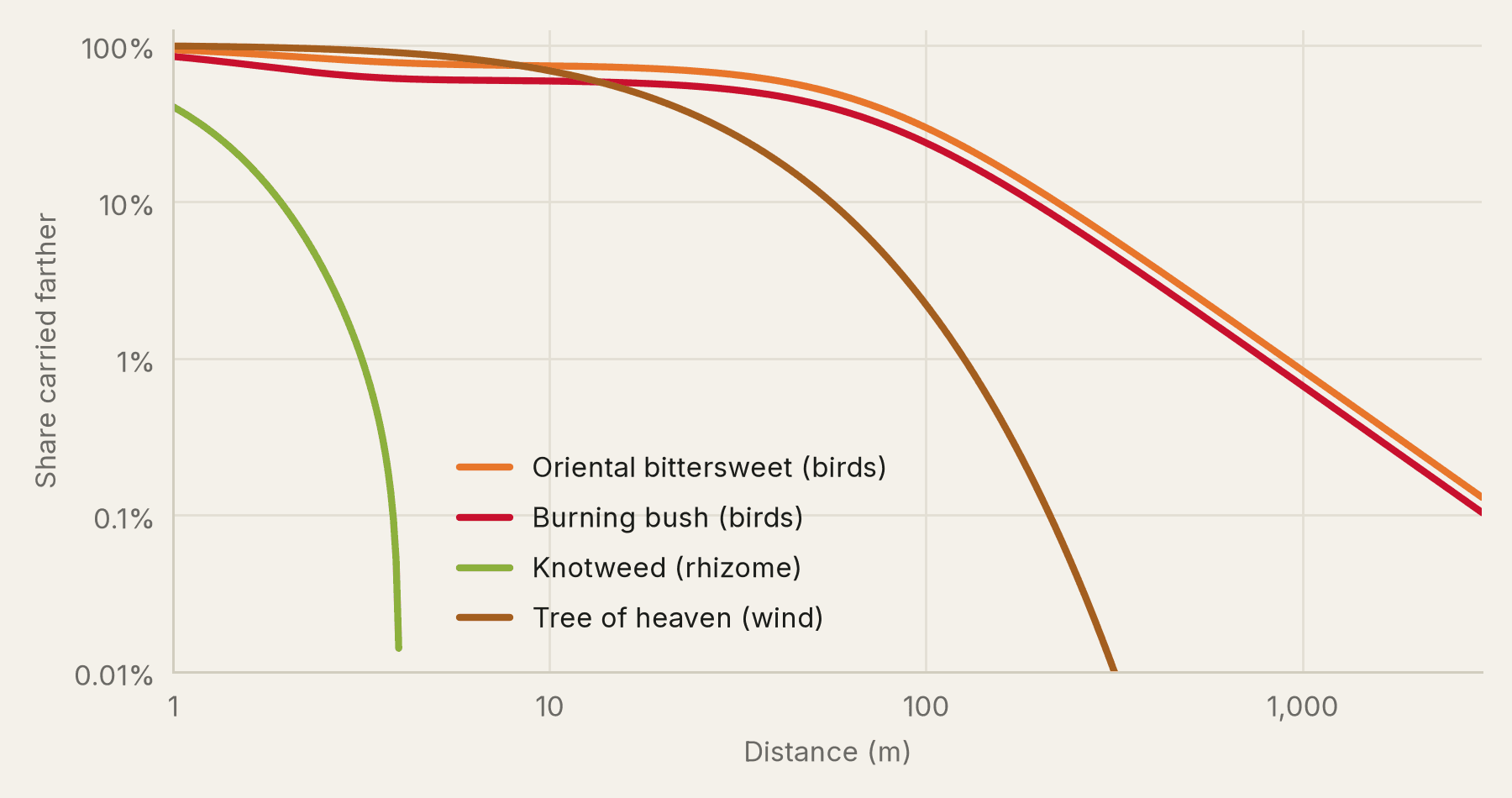
If nobody acts, Turning Mill Pond’s 18 surveyed patches are expected to cover 66,556 m² by 2031, and clearing its most valuable patch, a burning bush, this fall prevents 4,490 m² of that. On an Apple M5 Max the simulator runs 172 five-year simulations a second on a 400 × 400 grid, and in your browser it runs at about 0.6 times its native speed.
Learned habitat
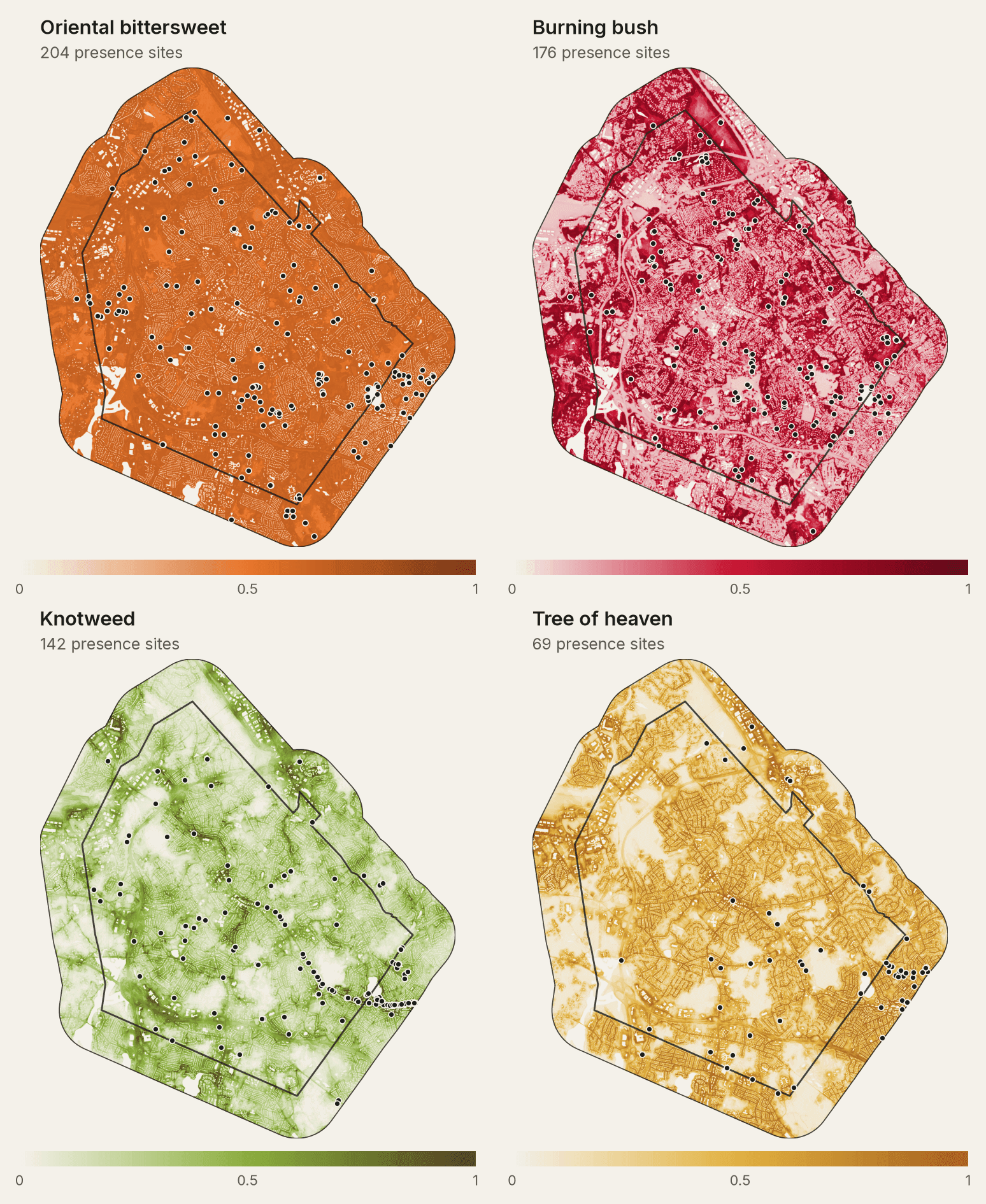
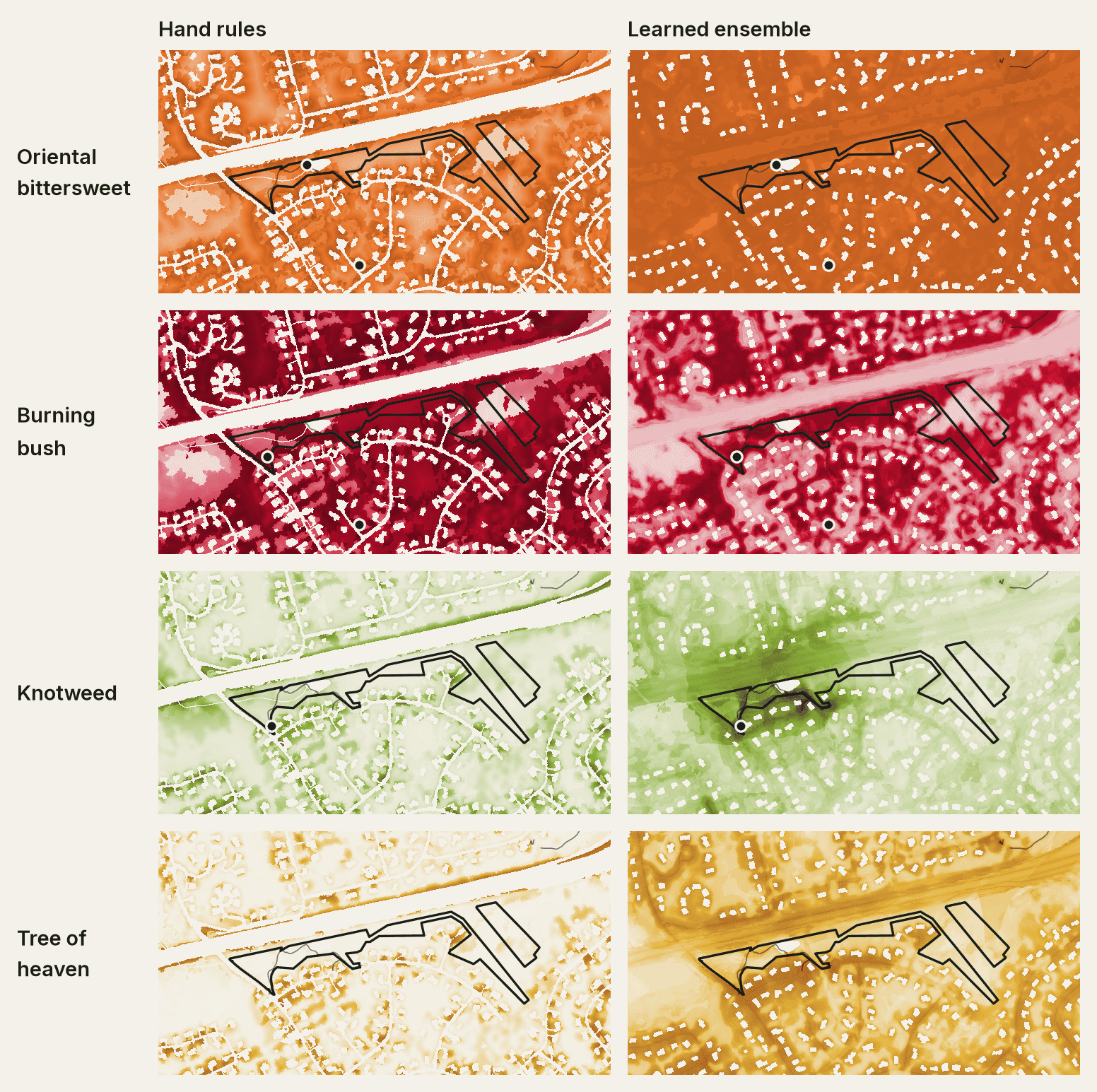
Where a seed can establish used to come from hand-written rules. Species distribution models now learn it from 22,271 iNaturalist plant records in and around Lexington, against a 2 m stack of lidar, terrain and land-cover covariates. Records of all plants, made by the same people on the same paths, serve as the background, so the models learn habitat rather than where people walk.
Town by town, statewide
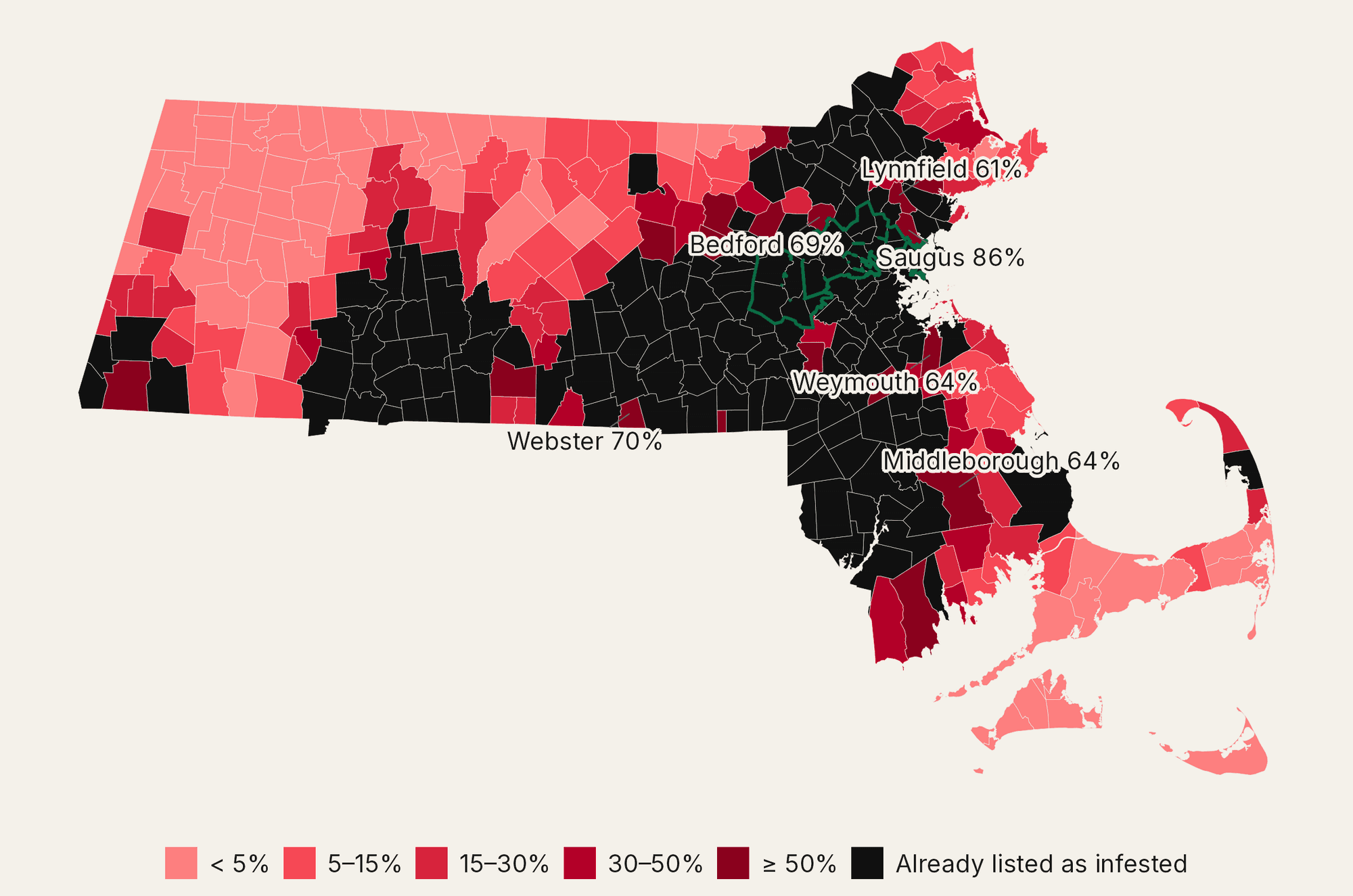
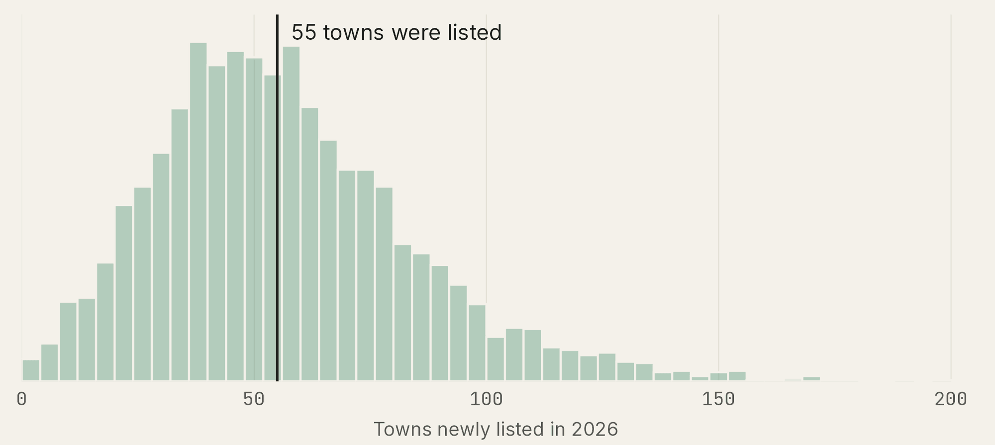
A Bayesian discrete-time hazard model, fit in Stan to the state’s listings from 2021 on, estimates each of Massachusetts’ 351 towns’ chance of a first spotted-lanternfly listing next year, from road and rail connectivity to infested towns, population, host trees and iNaturalist effort. It was tested prospectively: fit only through 2025, then scored on what happened in 2026.
13Seen on iNaturalist first
61Same year
58Listed by the state first
33No iNaturalist sighting
| Metric | Result | |
|---|---|---|
| AUC for 2026 listings | Ranking of the 241 at-risk towns, model fit through 2025 | 0.90 |
| Brier score | Accuracy of the 2026 probabilities; a constant rate scores 0.176 | 0.105 |
| New towns in 2026 | Predicted against observed | 57 vs 55 |
| New towns in 2027 | Expected first listings among the 186 towns not yet listed | 32 |
| Citizen science | Towns where iNaturalist saw it before the state listed it | 13 of 165 |
Spending scarce hours
A workday is a budget of volunteer-minutes. Each surveyed patch becomes a task worth the spread that clearing it prevents over five years, estimated by the simulator, and costing the walk in and out plus the person-minutes of work, matched to the skill it needs. Bittersweet is the slow one, done in three parts as on a real workday: the brush around the vines is cleared, each vine cut free and its roots pulled, and the cut vines piled beside the patch; at the end of the day everyone carries the piles to the trailhead; then they load the dumpster.
Volunteers work in groups of two to five, as real workdays do, never alone. Timefold Solver tries every way of splitting the crew, and for each it routes the groups along the property’s trails, solving a team orienteering problem with time windows in which a group shares the work at each patch. After the most prevented spread, it minimises everyone’s time on site, so groups finish together and, when the work worth doing runs out, the day ends early instead of leaving people standing around. The API simulates the chosen patches together, so overlapping spread isn’t counted twice, and compares the plan with three rules of thumb for the same groups, replayed exactly: largest patch first, nearest patch first, and random order.
The plan is the set of patches that prevents the most spread. Here is the area invaded in year 5 when the patches in are cleared now, and holds every set the crew can walk to and clear within its minutes . Today’s planner adds up single-patch values instead.
| Method | Prevented (m²) | Patches | Walking (min) |
|---|---|---|---|
| Random order | 1,650 | 5.2 | 96.8 |
| Nearest patch first | 1,911 | 5.8 | 51.8 |
| Largest patch first | 6,784 | 4.8 | 104.4 |
| Most value per minute | 7,214 | 6.4 | 88.7 |
| Optimized plan, 1 s | 7,435 | 6.6 | 89.9 |
| Optimized plan, 5 s (default) | 7,437 | 6.4 | 88.8 |
Real patches
On the real patches from my blind check, 18 at Turning Mill Pond and 7 at Wright Farm, every crew that follows the plan prevents more spread than the same crew clearing patches in trail order, the order the trail passes them.
| Crew | Planned (m²) | Trail order (m²) | Gain |
|---|---|---|---|
| Turning Mill Pond, 3 volunteers × 2 h | 28,558 | 19,277 | +48.1% |
| Turning Mill Pond, 5 volunteers × 3 h | 41,571 | 30,067 | +38.3% |
| Turning Mill Pond, 8 volunteers × 3 h | 54,006 | 46,591 | +15.9% |
| Wright Farm, 3 volunteers × 2 h | 16,554 | 9,675 | +71.1% |
| Wright Farm, 5 volunteers × 3 h | 30,774 | 21,891 | +40.6% |
| Wright Farm, 8 volunteers × 3 h | 39,310 | 31,130 | +26.3% |
Try it now by planning a workday for a sample crew or explore every invasive patch on the map.
Sources and reproducibility
- Spotted lanternfly town listings from the Massachusetts Department of Agricultural Resources, queried 12 Oct 2026
- Town boundaries, rail and highways from MassGIS, with population from the 2020 Census
- Sightings, plant records and training photos from iNaturalist, under CC0, CC BY and CC BY-NC licenses
- Canopy and terrain from USGS 3DEP lidar, 2021
- Land cover, wetlands and water from MassGIS Land Cover/Land Use 2016, MassDEP wetlands and MassGIS hydrography
- Conservation land from MassGIS Protected and Recreational OpenSpace and the Town of Lexington’s parcels
- Trails and buildings from the Town of Lexington and OpenStreetMap contributors
- Elevation for the 3D maps from Mapzen Terrain Tiles on AWS Open Data, built from USGS 3DEP
- Field observations from Lexington steward patrols, with geotagged photos